OSPCMRI Processing
Please contact Conan Chen for any questions about this page.
OSPCMRI Processing Overview
To process OSPCMRI data acquired from the CFMRI Prisma scanner, this pipeline can be run on any Linux or Mac system with MATLAB, AFNI and dcm2niix installed.
Software Requirements
MATLAB- version R2023b or newer (requires volume viewer with the Scissors tool, which is only available in R2023b+)AFNI- version AFNI_23.1.00 or newer (older versions may work but are untested)dcm2niix- v1.0.20240202 or newer (older versions may work but are untested)
To check for AFNI command-line access and version:
# Should return a path like /Users/username/abin/afni
which afni

# Should return output like
#Precompiled binary macos_10.12_local: Apr  7 2023 (Version AFNI_23.1.00 'Publius Helvius Pertinax')
afni --version
To check for dcm2niix command-line access and version:
# Should return a path like /Users/username/bin/dcm2niix
which dcm2niix

# Should return output like:
# Chris Rorden's dcm2niiX version v1.0.20240202  (JP2:OpenJPEG) (JP-LS:CharLS) Clang12.0.0 ARM (64-bit MacOS)
# v1.0.20240202
dcm2niix --version
Computers/Servers
This pipeline can be potentially setup on your lab’s server (please contact Conan Chen for assistance). It is also available to users on fmri1 or fmri3.
Setup
Subject-Specific Script
This setup script can be configured either using a simple text editor (e.g. notepad, textedit, Sublime) or in MATLAB. Setup consists of configuring a setup script, where you specify paths for processing.
%% SampleSetup_SingleSubject
% Example setup script for running OSPCMRI processing on a single subject.

% Clear variables and close any figures.
clear
close all hidden

% Add path to the processing code repository
addpath('/path/to/repo/OSPCMRI');

% Dataset directory
basedir = '/path/to/subjectfolder/';

% TOF DICOM directory
tofdir = [basedir '0006_tof_fl3d_tra_p2_Slabs4_PF66/'];

% Localizer DICOM directory
locdir = [basedir '0001_localizer_64ch/'];

% Specifying OSPCMRI datasets
idataset = 1;
datasets(idataset).ospcmridir = [basedir '0015_OSPCMRI_sag_in-plane_FA10_Venc100_left_P/'];
datasets(idataset).tofdir = tofdir;
datasets(idataset).locdir = locdir;

idataset = 2;
datasets(idataset).ospcmridir = [basedir '0037_OSPCMRI_sag_in-plane_FA10_Venc100_right_P/'];
datasets(idataset).tofdir = tofdir;
datasets(idataset).locdir = locdir;

%{
% Specify additional OSPCMRI datasets, if present.
idataset = 3;
datasets(idataset).ospcmridir = [basedir '0037_OSPCMRI_sag_in-plane_FA10_Venc100_right_P/'];
datasets(idataset).tofdir = tofdir;
datasets(idataset).locdir = locdir;
%}

% Looping over OPSCMRI datasets.
for idataset = 1:length(datasets)

    % Calling the processing function.
    procOSPCMRI( ...
        datasets(idataset).ospcmridir ...      % OSPCMRI DICOM directory
        , datasets(idataset).tofdir ...        % TOF DICOM directory
        , locdir=datasets(idataset).locdir ... % localizer DICOM directory
        );

    % Add any optional processing flags on a new line (example below):
    %
    %procOSPCMRI( ...
    %    datasets(idataset).ospcmridir ...      % OSPCMRI DICOM directory
    %    , datasets(idataset).tofdir ...        % TOF DICOM directory
    %    , locdir=datasets(idataset).locdir ... % localizer DICOM directory
    %    , flag_overwrite=1 ...                 % overwrite outputs
    %    );
    %

end % idataset
Multiple-Subject (Looping) Script
The pipeline can also be run by looping over many subjects. This setup approach can be much more efficient if you are processing many subjects at once. This may let you avoid specifying tons of individual setup scripts, especially if many subjects are already organized in a well-defined directory structure.
%% SampleSetup_MultipleSubjects
% Example setup script for running OSPCMRI processing on multiple subjects
% over a loop.

% Clear variables and close any figures.
clear
close all hidden

% Add path to the processing code repository
addpath('/path/to/repo/OSPCMRI');


%%%%% ==== Code to automatically create a subjects struct array ==== %%%%%
% ... code depends on directory structure
%%%%% === End code to automatically create a subjects struct array == %%%%%


% Looping over subjects for processing.
for isubject = 1:length(subjects)

    % For printing progress.
    fprintf('Processing isubject %.f | datadir = %s \n', isubject, subjects(isubject).datadir);

    % Looping over OPSCMRI datasets.
    for idataset = 1:length(subjects(isubject).datasets)

        datadir = subjects(isubject).datadir;
        ospcmridir = [datadir subjects(isubject).datasets(idataset).ospcmridir];
        tofdir = [datadir subjects(isubject).datasets(idataset).tofdir];
        locdir = [datadir subjects(isubject).datasets(idataset).locdir];

        % Calling the processing function.
        procOSPCMRI( ...
            ospcmridir ...      % OSPCMRI DICOM directory
            , tofdir ...        % TOF DICOM directory
            , locdir=locdir ... % localizer DICOM directory
            );

        % Add any optional processing flags on a new line (example below):
        %
        %procOSPCMRI( ...
        %    ospcmridir ...      % OSPCMRI DICOM directory
        %    , tofdir ...        % TOF DICOM directory
        %    , locdir=locdir ... % localizer DICOM directory
        %    , flag_overwrite=1 ...                 % overwrite outputs
        %    );
        %

    end % idataset

end % isubject
Contact Conan Chen for assistance setting up a Multiple-Subject setup script.
Optional Flags
You can specify optional inputs/flags directly in the setup script, in the call to procOSPCMRI. Listed below are the optional inputs along with a brief description.
%  Optional Directories:
%   locdir              localizer DICOM directory path, used for performing
%                       an optional Rx check - see flag_checkRx
%   procdir             the processed directory where pipeline outputs
%                       will be generated; defaults to a folder named as
%                       the OSPCMRI directory suffixed by '_Processed'
%
%  Overwriting Flags:
%   flag_overwrite      [0]/1 - flag to overwrite procdir by removing the
%                       directory first if it already exists
%   flag_reuseTOFmask   [0]/1 - flag to look inside a pre-existing
%                       processed directory, and re-use prexisting TOF mask
%                       from results.mat for subsequent processing
%
%  Publishing flags:
%   flag_publish        0/[1] - publish an HTML summary report
%   flag_publishcode    [0]/1 - include code in HTML summary report
%   flag_publishopen    0/[1] - open the report after processing
%   flag_makefigs       0/[1] - make figures throughout processing
%
%
%  Rx Checking Flags:
%   flag_checkRx        0/[1] - use the localizer, TOF and OSPCMRI scans to
%                       create an image checking their relative positioning
%
%  TOF Processing Flags:
%   flag_itermask       0/[1] - flag for iteratively removing voxels from
%                       the vessel mask
%   flag_manualBP       [0]/1 - flag for manually identifying the carotids
%                       branch point
%   flag_padnslices'    [5]   - specifies number of zero-pad slices on each
%                       side of OSPCMRI; this effectively determines the
%                       extents of the TOF box to examine
%
%  OSPCMRI Processing Flags:
%   flag_corrmask'      0/[1] - flag for refining OSPCMRI mask by removing
%                       voxels that are poorly correlated with the
%                       reference (mean) OSPCMRI waveform
%   flag_corrmaskthresh [0.8] - the correlation exclusion threshold, below
%                       which axial OSPCMRI waveforms will be excluded
%   flag_corritermask   [0]/1 - flag for iteratively removing voxels from
%                       the vessel mask; only considered if flag_corrmask=1
%   flag_smooth         0/[1] - flag for smoothing OSPCMRI waveforms
%   flag_upsample       0/[1] - flag for upsampling OSPCMRI waveforms
%   flag_WLS            [0]/1 - flag for using weighted least squares
%                       (weighted by number of voxels) when fitting line
%                       for PWV
%   flag_robust         0/[1] - flag for using robust least squares when
%                       fitting line for PWV
%   flag_censor         0/[1] - flag for removing outliers when fitting
%                       line for PWV
%   flag_censoriter     0/[1] - flag for iteratively removing outliers when
%                       fitting line for PWV; only used if flag_censor=1
%
Pipeline Steps
Initiating the Pipeline
Launch MATLAB from your terminal (which should have command line access to AFNI). This will ensure your MATLAB instance also has command-line access to AFNI and dcm2niix, which it will need for several processing steps. Then simply run the setup script.
Checking the Prescription
The first figure produced will look like below, serving as a quick visual check on the OSPCMRI prescription. The grayscale image in the background is the sagittal localizer resampled to a low-resolution grid. The cyan box outline represents the TOF prescription, and the yellow outline represents the OSPCMRI prescription.
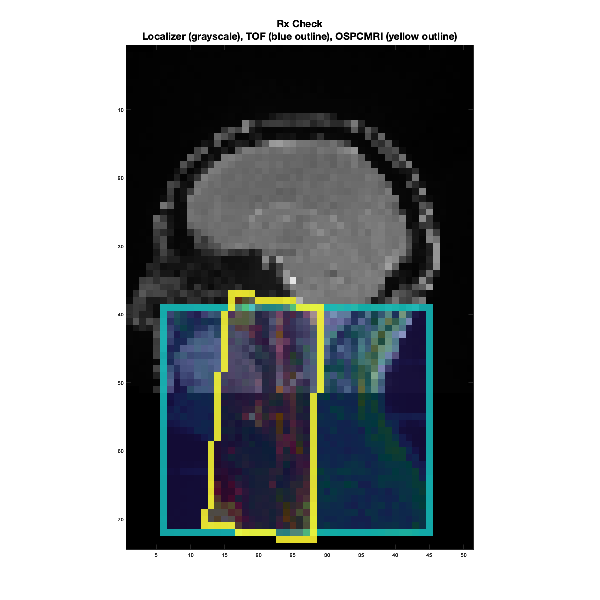
Example of a “good” prescription check. The TOF roughly covers the neck area below the cerebellum, which is generally the level where we expect the target CCA-ICA segment for most subjects.
Bad examples:
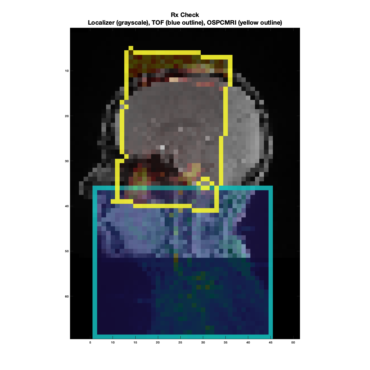
Example of a “bad” prescription check. The TOF coverage is good, but the OSPCMRI was prescribed too superiorly, way into the brain, missing the target CCA-ICA segment altogether.
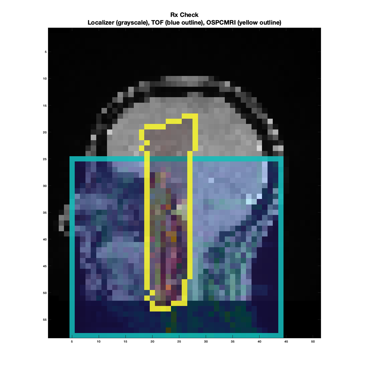
Example of a “bad” prescription check. Both the TOF and OSPCMRI prescriptions are too high/superior into the brain, missing the target CCA-ICA segments altogether.
If you see that the prescription is totally off, you thus have an early indicator that the dataset will need to be excluded from further analysis.
TOF vessel masking (semi-automated)
The video below shows a simple example of vessel masking, demonstrating using the “Scissors” tool to refine the vessel mask, and the “Keep max-overlap component” to assist with removing any minor unconnected components.
Ultimately, aim for a vessel mask that cleanly shows the CCA, ICA, and ECA, like in the example below.
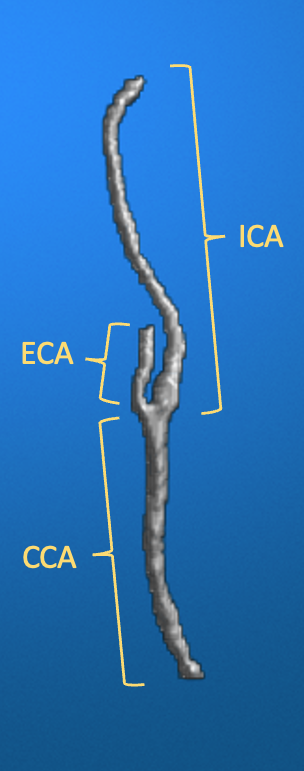
Example of a “good” vessel mask that clearly shows the CCA, ICA and ECA after the semi-automated masking step.
For this pipeline, cut the ECA branch so that it is shorter than the ICA branch, while still remaining a distinguishable branch (i.e. do not remove it altogether, as the ECA will be used to identify the branching point, which in turn is used to compute PI and RI values for CCA and ICA). Given this vessel mask, the CCA-ICA segment will be automatically detected as the path that connects the furthest two endpoints in the inferior-superior directions. The ECA branch will be assumed as the largest branch outside of the CCA-ICA path.
The video below shows a more complicated example of vessel masking, demonstrating using the “Reset” button to restart the vessel masking state, adjusting the TOF threshold until the target CCA/ICA segment can be clearly identified, and again using the “Scissors” tool and “Keep max-overlap component” button to refine the vessel mask. Also demonstrated is toggling the “Show sub-threshold data” checkbox to better visualize the working vessel mask.
Once you are satisfied with the vessel mask, click “TOF masking complete”. This will complete this step and proceed with the remainder of the pipeline.
Remainder of the pipeline (automated)
The remainder of the pipeline is automated, consisting of several TOF processing steps:
Skeletonizing the vessel mask.
Identifying the CCA, ICA and ECA segments.
Identifying the carotids branch point (where CCA splits into ICA and ECA)
Pruning ECA (and any other minor or spurious branches) to produce the CCA-ICA segment of interest.
Computing the distance along the vessel, starting from the bottom endpoint and ending at the top endpoint.
Using the TOF-derived CCA-ICA mask to produce an initial OSPCMRI vessel mask.
Attention
Note, however, that the pipeline may prompt you to manually indicate the carotids branch point in the rare cases that it cannot be identified automatically.
And several OSPCMRI processing steps:
Retrieve the OSPCMRI data and initial OSPCMRI mask
Interpolate missing/outlier timepoints
Smooth waveforms (Optional)
Refining OSPCMRI mask exclude non-positive voxels
Refining OSPCMRI mask by correlation filter (Optional)
Bin (average) OSPCMRI waveforms by their locations along the vessel
Normalize all waveforms between 0 and 1
Compute Pulse Wave Velocity (PWV)!
Compute PI and RI for the CCA and ICA
Generate waves figure
Writing results to file
Outputs
Files in the Processed Directory
Below are the outputs nested under the *_processed/ folder for a given OSPCMRI processing run:
0015_OSPCMRI_sag_in-plane_FA10_Venc100_left_P_processed % ls -1
1_localizer_64ch_i00001.json                                     # axial localizer json
1_localizer_64ch_i00001.nii                                      # axial localizer NIFTI
1_localizer_64ch_i00006.json                                     # sagittal localizer json
1_localizer_64ch_i00006.nii                                      # sagittal localizer NIFTI
1_localizer_64ch_i00011.json                                     # coronal localizer json
1_localizer_64ch_i00011.nii                                      # coronal localizer NIFTI
15_OSPCMRI_sag_in-plane_FA10_Venc100_left_P_ph.json              # OSPCRMI json
15_OSPCMRI_sag_in-plane_FA10_Venc100_left_P_ph.nii               # OSPCMRI NIFTI
15_OSPCMRI_sag_in-plane_FA10_Venc100_left_P_ph_RAI.nii           # reoriented to RAI (right-anterior-inferior) via AFNI
15_OSPCMRI_sag_in-plane_FA10_Venc100_left_P_ph_RAI_pad.nii       # zero-padded with additional slices
15_OSPCMRI_sag_in-plane_FA10_Venc100_left_P_ph_RAI_pad_rs.nii    # resampled to 1mm isotropic resolution
6_tof_fl3d_tra_p2_Slabs4_PF66.json                               # TOF json
6_tof_fl3d_tra_p2_Slabs4_PF66.nii                                # TOF NIFTI
6_tof_fl3d_tra_p2_Slabs4_PF66_warp.nii                           # warped to the OSPCMRI oblique orientation
6_tof_fl3d_tra_p2_Slabs4_PF66_warp_rs.nii                        # resample to 1mm isotropic resolution
CheckRx_LocSag_lowres.nii                                        # checking the Rx: low-res sagittal localizer
CheckRx_LocSag_lowres_pad2TOF.nii                                # checking the Rx: padding to cover/include the TOF FOV
CheckRx_OSPCMRI_dbq.nii                                          # OSPCMRI, deobliqued to cardinal orientation
CheckRx_OSPCMRI_dbq_RAI.nii                                      # reorienting to RAI
CheckRx_OSPCMRI_dbq_resampled.nii                                # resampled to the low-res
CheckRx_TOF_resampled.nii                                        # TOF, resampled to the low-res
params_struct.mat                                                # MATLAB file containing the processing flags/parameters
publish_procOSPCMRI_script.m                                     # copy of the processing script
results.txt                                                      # results in text format
results.json                                                     # results in json format
results.mat                                                      # MATLAB struct of the processing results
Report/                                                          # subfolder containing the html report
Results Files
The results.txt file is a two-column text file with the main results.
VariableName        Value
patient_ID          <SubjectID>
patient_age_Y       <##>
patient_sex         <M/F>
patient_height_m    1.7272034566667
patient_weight_lbs  88.4505234015
RR_mean_ms          1110
RR_stdv_ms          360
PWV_MUSA_mps        5.45916154412884
PWVpval_MUSA        1.78054573234104e-10
PWV_TTF_mps         12.7095120899872
PWVpval_TTF         0.00178606108218448
PWV_CXCORR_mps      5.59672744563534
PWVpval_CXCORR      7.96187471108059e-20
PI_CCA              1.34778799717965
PI_ICA              1.44859280645189
RI_CCA              2.95786033222646
RI_ICA              1.22547765544041
scan_name           OSPCMRI_sag_in-plane_FA10_Venc100_left
scan_side           left
The results.json file contains the same information but in json format.
The results.mat file is a MATLAB save-file of a struct with all of the processing outputs for the given dataset.
QA Summary Report
At the end of the processing, a QA summary report will be automatically generated and opened in your web browser. The report itself is located within the *_processed/Report folder as the publish_procOSPCMRI_script.html file. The images in the same location correspond to the various images shown throughout the report.
The report summarizes every proessing step of the pipeline, along with every figure generated in the process. It provides a comprehensive way to quickly check the quality of every processing step and help troubleshoot any issues with the PWV outputs.
This download link provides a sample OSPCMRI Processing report on data collected at CFMRI. After unzipping the file, the report given by publish_procOSPCMRI_script.html can be opened in a web browser.
The video below scrolls through this example report.